As part of the NFL’s technology conference held last week, I presented to club staffers various approaches on how R could be used to explore NFL data. Here’s a slightly abridged version. This specific audience featured both novice and expert R users. Given that a semester’s long course would be needed to truly cover the breadth of how R could help explore football, note that this particular document is more an overview than anything else. Finally, most of the code is not meant to be run from an outsiders’ perspective, and instead uses a few internal databases. I’m sharing publicly in case it spurs any ideas for analysis or visualization.
Summary of session
Tidyverse and NFL analytics
Sample visualizations using
ggplot2Big Data Bowl insight
Tidyverse and NFL analytics
Packages
Favorite packages to use for manipulation, tidying, data viz, analysis
tidyverse: Data manipulation and graphinglubridate: Handling datesggbeeswarm: Fun plotsggridges: Fun plotsgganimate: Fun animationstidyr: Tidy data (wide to long/long to wide)nflscrapr: Public win probabilities and expected pointscaret: Machine learning toolslme4: Statistical modelingteamcolors: Team specific hex codes
#install.packages("tidyverse")
library(tidyverse)
library(lubridate)
library(beeswarm)
library(gganimate)
library(ggridges)
library(tidyr)
Reading in data
library(tidyverse)
df_games <- read_csv("prodb/dbo.Game.csv")
df_plays <- read_csv("prodb/dbo.VideoDirectorReport.csv")
Joining data sets
Online cheat-sheet: https://stat545.com/bit001_dplyr-cheatsheet.html
left_join:
inner_join:
right_join:
anti_join:
Data manipulation using the tidyverse
Online cheat-sheet: https://www.rstudio.com/wp-content/uploads/2015/02/data-wrangling-cheatsheet.pdf
Key commands:
select()head()tail()filter()
df_plays_keep <- df_plays %>%
  filter(HomeTeamFile == 1) %>%
  select(GameKey, HomeClubCode, VisitorClubCode, Quarter,
        PossessionTeam, PlayNullifiedByPenalty,
        SpecialTeamsPlayType, PlayResult, Down, Distance, PlayDescription)
df_games <- df_games %>% select(GameKey, Season, Season_Type, Week, LeagueType)

df_plays_keep <- df_plays_keep %>% left_join(df_games, by = c("GameKey" = "GameKey"))
df_plays_keep %>% head()
## # A tibble: 6 x 15
## GameKey HomeClubCode VisitorClubCode Quarter PossessionTeam
## <int> <chr> <chr> <int> <chr>
## 1 745 TEN PIT 2 TEN
## 2 745 TEN PIT 2 TEN
## 3 745 TEN PIT 4 PIT
## 4 745 TEN PIT 4 PIT
## 5 745 TEN PIT 4 PIT
## 6 745 TEN PIT 4 PIT
## # … with 10 more variables: PlayNullifiedByPenalty <chr>,
## # SpecialTeamsPlayType <chr>, PlayResult <int>, Down <int>,
## # Distance <int>, PlayDescription <chr>, Season <int>,
## # Season_Type <chr>, Week <int>, LeagueType <chr>df_plays_keep %>% tail()## # A tibble: 6 x 15
## GameKey HomeClubCode VisitorClubCode Quarter PossessionTeam
## <int> <chr> <chr> <int> <chr>
## 1 57464 NE BUF 3 BUF
## 2 57469 SF JAX 2 JAX
## 3 57466 NYJ LAC 1 LAC
## 4 57462 CIN DET 4 DET
## 5 57442 IND DEN 4 DEN
## 6 57467 TEN LA 4 LA
## # … with 10 more variables: PlayNullifiedByPenalty <chr>,
## # SpecialTeamsPlayType <chr>, PlayResult <int>, Down <int>,
## # Distance <int>, PlayDescription <chr>, Season <int>,
## # Season_Type <chr>, Week <int>, LeagueType <chr>- More
filter(): Categorical variables
df_plays_keep %>%
  filter(Down == 4, Quarter == 1, Distance == 12,
         PlayNullifiedByPenalty == "N", SpecialTeamsPlayType == "NULL")
## # A tibble: 4 x 15
## GameKey HomeClubCode VisitorClubCode Quarter PossessionTeam
## <int> <chr> <chr> <int> <chr>
## 1 26558 NE BUF 1 BUF
## 2 29406 CLV BUF 1 BUF
## 3 54993 CIN NO 1 CIN
## 4 29772 GB DET 1 GB
## # … with 10 more variables: PlayNullifiedByPenalty <chr>,
## # SpecialTeamsPlayType <chr>, PlayResult <int>, Down <int>,
## # Distance <int>, PlayDescription <chr>, Season <int>,
## # Season_Type <chr>, Week <int>, LeagueType <chr>df_plays_keep <- df_plays_keep %>%
filter(Season_Type == "Reg", Season >= 2005, Season <= 2018, LeagueType == "NFL")What data set did we create?
arrange()
df_plays_keep %>%
  filter(PossessionTeam == "MIN", Season == 2018) %>%
  arrange(-PlayResult) %>%
  head()
## # A tibble: 6 x 15
## GameKey HomeClubCode VisitorClubCode Quarter PossessionTeam
## <int> <chr> <chr> <int> <chr>
## 1 57812 MIN CHI 2 MIN
## 2 57586 GB MIN 4 MIN
## 3 57607 MIN BUF 2 MIN
## 4 57694 MIN DET 2 MIN
## 5 57640 PHI MIN 3 MIN
## 6 57668 NYJ MIN 3 MIN
## # … with 10 more variables: PlayNullifiedByPenalty <chr>,
## # SpecialTeamsPlayType <chr>, PlayResult <int>, Down <int>,
## # Distance <int>, PlayDescription <chr>, Season <int>,
## # Season_Type <chr>, Week <int>, LeagueType <chr>What plays are these??
mutate()
df_plays_keep <- df_plays_keep %>%
  mutate(is_first_down = PlayResult >= Distance,
         scrimmage_play = SpecialTeamsPlayType == "NULL")

df_plays_keep %>%
  filter(PossessionTeam == "MIN", Season == 2018, Down == 4, scrimmage_play, Quarter == 1)
## # A tibble: 4 x 17
## GameKey HomeClubCode VisitorClubCode Quarter PossessionTeam
## <int> <chr> <chr> <int> <chr>
## 1 57694 MIN DET 1 MIN
## 2 57686 MIN NO 1 MIN
## 3 57741 MIN GB 1 MIN
## 4 57651 MIN ARZ 1 MIN
## # … with 12 more variables: PlayNullifiedByPenalty <chr>,
## # SpecialTeamsPlayType <chr>, PlayResult <int>, Down <int>,
## # Distance <int>, PlayDescription <chr>, Season <int>,
## # Season_Type <chr>, Week <int>, LeagueType <chr>, is_first_down <lgl>,
## # scrimmage_play <lgl>What do these four plays represent?
group_by()summarize()
df_plays_keep %>%
  filter(scrimmage_play, Season == 2018) %>%
  group_by(PossessionTeam) %>%
  summarise(ave_yds_gained = mean(PlayResult)) %>%
  arrange(-ave_yds_gained) %>%
  head()
## # A tibble: 6 x 2
## PossessionTeam ave_yds_gained
## <chr> <dbl>
## 1 KC 6.25
## 2 LA 6.04
## 3 ATL 5.78
## 4 PIT 5.76
## 5 TB 5.70
## 6 LAC 5.67Identify the leaderboard above:
df_plays_keep %>%
  filter(scrimmage_play) %>%
  group_by(PossessionTeam, Season) %>%
  summarise(ave_yds_gained = mean(PlayResult)) %>%
  arrange(-ave_yds_gained) %>%
  head()
## # A tibble: 6 x 3
## # Groups: PossessionTeam [6]
## PossessionTeam Season ave_yds_gained
## <chr> <int> <dbl>
## 1 ATL 2016 6.29
## 2 NO 2011 6.26
## 3 KC 2018 6.25
## 4 GB 2011 6.08
## 5 LA 2018 6.04
## 6 ARZ 2015 5.96Identify the leaderboard above:
df_plays_keep %>%
  filter(scrimmage_play) %>%
  group_by(PossessionTeam, Season) %>%
  summarise(ave_yds_gained = mean(PlayResult)) %>%
  arrange(-ave_yds_gained) %>%
  tail()
## # A tibble: 6 x 3
## # Groups: PossessionTeam [5]
## PossessionTeam Season ave_yds_gained
## <chr> <int> <dbl>
## 1 HST 2005 3.81
## 2 CIN 2008 3.80
## 3 ARZ 2012 3.74
## 4 SF 2005 3.61
## 5 SF 2007 3.59
## 6 OAK 2006 3.50Identify the leaderboard above:
Data visualization
Sample Q1: How often do teams go for it on 4th-short in each season?
fourth_down_rates <- df_plays_keep %>%
  filter(Down == 4, Distance <= 2) %>%
  group_by(PossessionTeam, Season) %>%
  summarise(go_forit_rate = mean(scrimmage_play),
            n_chances = n())


fourth_down_rates %>%
  arrange(-go_forit_rate) %>%
  head()
## # A tibble: 6 x 4
## # Groups: PossessionTeam [6]
## PossessionTeam Season go_forit_rate n_chances
## <chr> <int> <dbl> <int>
## 1 JAX 2013 0.692 26
## 2 BUF 2018 0.688 16
## 3 NE 2007 0.682 22
## 4 CLV 2017 0.667 15
## 5 MIN 2018 0.654 26
## 6 BLT 2018 0.65 20fourth_down_rates %>%
arrange(go_forit_rate) %>%
head()## # A tibble: 6 x 4
## # Groups: PossessionTeam [6]
## PossessionTeam Season go_forit_rate n_chances
## <chr> <int> <dbl> <int>
## 1 BUF 2012 0.05 20
## 2 CIN 2007 0.0526 19
## 3 SL 2015 0.0588 17
## 4 CAR 2006 0.0714 28
## 5 ATL 2012 0.0938 32
## 6 MIN 2005 0.1 30library(ggbeeswarm)
fourth_down_rates %>%
ggplot(aes(x = Season, y = go_forit_rate, fill = go_forit_rate)) +
geom_quasirandom(pch = 21, size = 3) +
scale_fill_viridis_c("", guide = FALSE) +
theme_classic(15) +
scale_x_continuous(labels = 2005:2018, breaks = 2005:2018) +
scale_y_continuous(labels = scales::percent) +
labs(title = "Go-for-it rate, 4th-1 or 4th-2", y = "", x = "")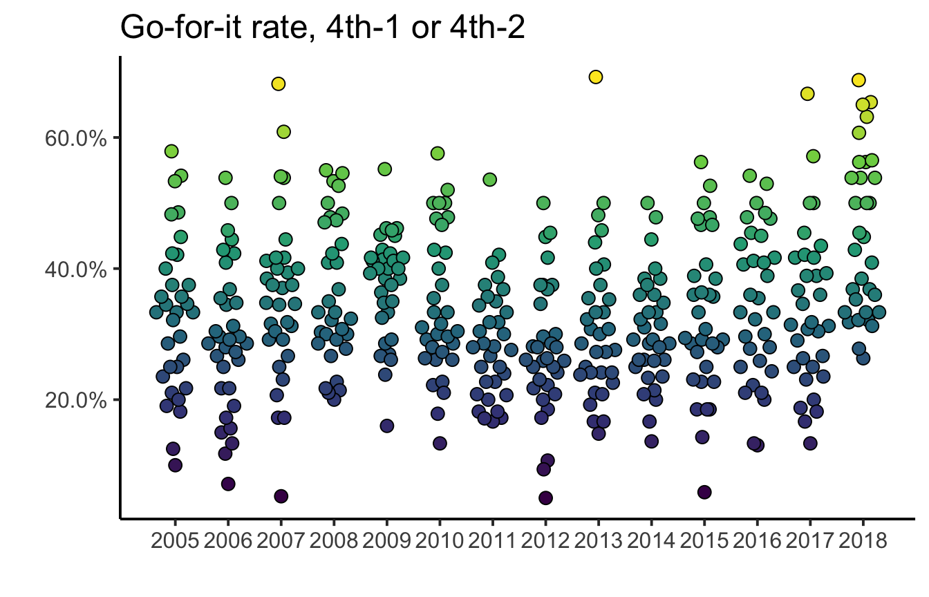
Sample Q2: What’s going on on the punt play?
df_punts_keep <- df_plays %>%
  filter(HomeTeamFile == 1, SpecialTeamsPlayType == "Punt"|SpecialTeamsPlayType == "Punt Return") %>%
  select(GameKey, HomeClubCode, VisitorClubCode, Quarter, KickoffResult,
        PossessionTeam, PlayNullifiedByPenalty,
        SpecialTeamsPlayType, PlayResult, Down, Distance, PlayDescription)

df_punts_keep <- df_punts_keep %>% left_join(df_games, by = c("GameKey" = "GameKey"))

## Penalty rate on punt plays using `grepl`
df_punts_keep %>%
  mutate(is_penalty = grepl("PENALTY", PlayDescription)) %>%
  summarise(p_rate = mean(is_penalty))
## # A tibble: 1 x 1
## p_rate
## <dbl>
## 1 0.138df_punts_keep %>%
filter(Season >= 2001) %>%
ggplot(aes(Season, fill = KickoffResult)) +
geom_bar(position = "fill") +
scale_fill_brewer(palette = "Set1") +
scale_y_continuous(labels = scales::percent, "Rate") +
labs(title = "Punt outcomes over time")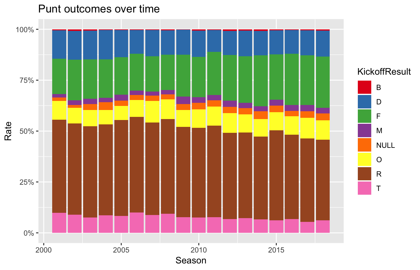
Other charts of interest
Examples from league office
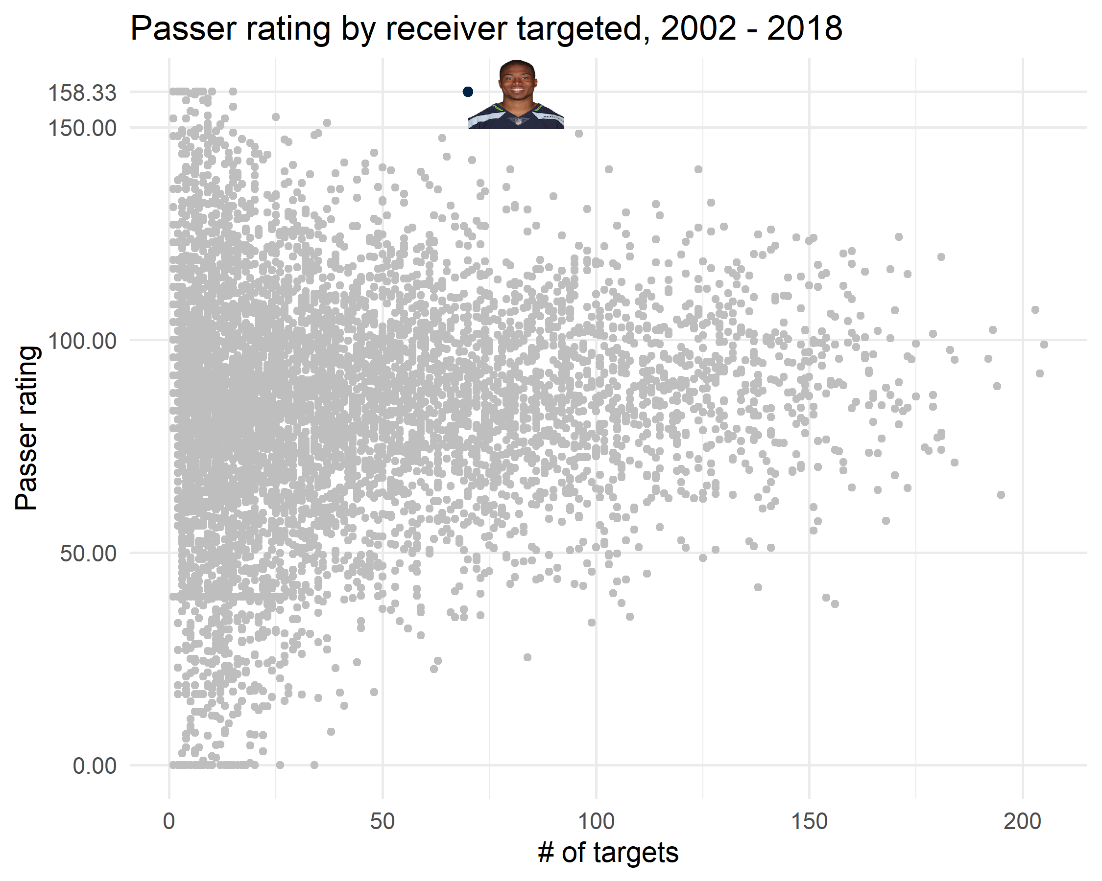
- Tyler Lockett funnel plot
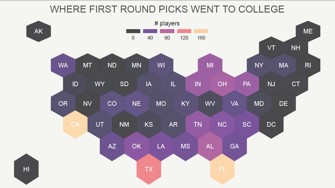
- Maps
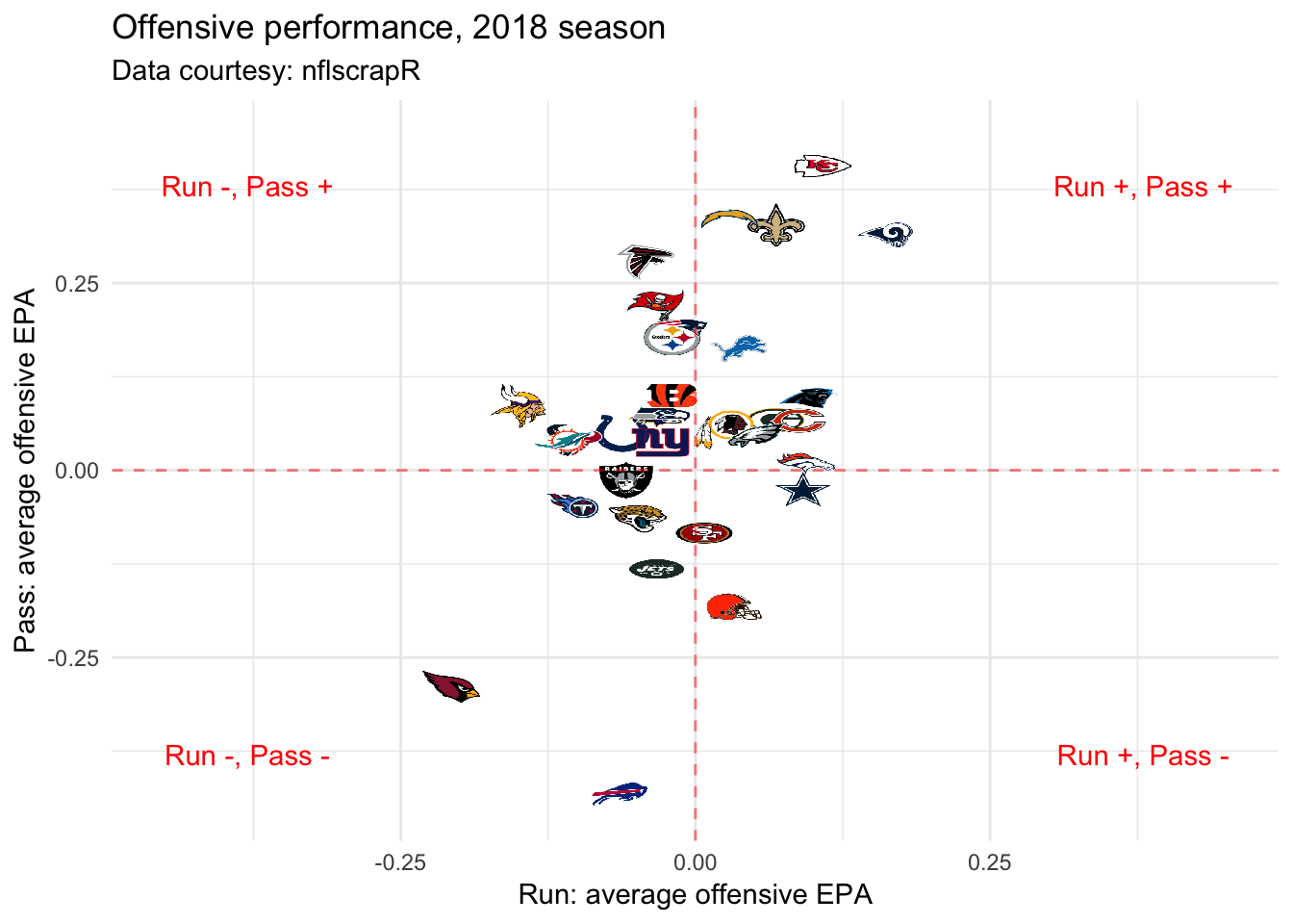
- Team logos with
ggimage: link
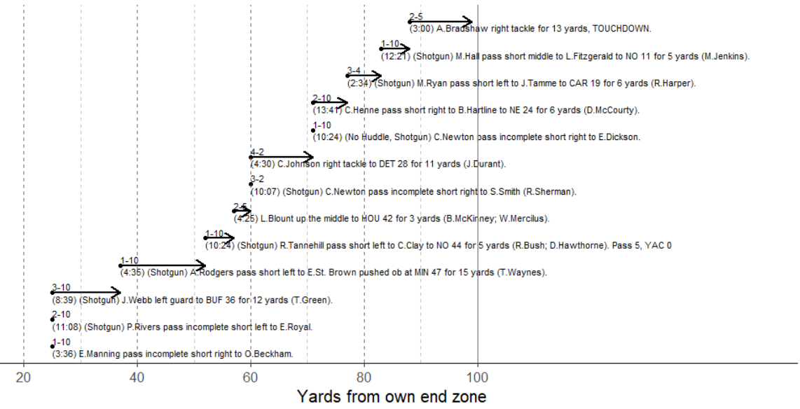
- Competition committee work: resampling plays to estimate overtime outcomes
What can we do with Next Gen Stats?
General processes for NGS data
- Start small. Identify play-type of interest and find 5-10 examples using
playId/gameId - Scrape data using https://docs.ngs.nfl.com and personal credentials
- Build animation/summary metrics within the sample of plays
- Re-center data using
playDirection - Re-orgin data using location where (player/ball) started
- Cross-check with video
- Expand across larger sample of plays
- Sample large sample of plays to cross-check for accuracy
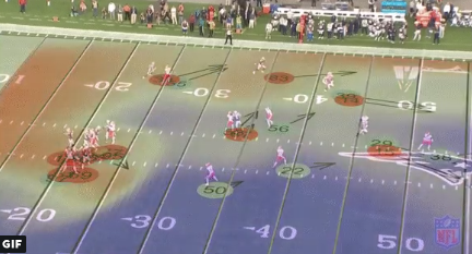
Play animation
file_tracking <- "https://raw.githubusercontent.com/nfl-football-ops/Big-Data-Bowl/master/Data/tracking_gameId_2017090700.csv"
tracking_example <- read_csv(file_tracking)

file_game <- "https://raw.githubusercontent.com/nfl-football-ops/Big-Data-Bowl/master/Data/games.csv"
games_sum <- read_csv(file_game)

file_plays <- "https://raw.githubusercontent.com/nfl-football-ops/Big-Data-Bowl/master/Data/plays.csv"
plays_sum <- read_csv(file_plays)

tracking_example_merged <- tracking_example %>% inner_join(games_sum) %>% inner_join(plays_sum)

example_play <- tracking_example_merged %>% filter(playId == 938)
example_play %>% select(playDescription) %>% slice(1)

library(gganimate)
library(cowplot)

## General field boundaries
xmin <- 0
xmax <- 160/3
hash.right <- 38.35
hash.left <- 12
hash.width <- 3.3


## Specific boundaries for a given play
ymin <- max(round(min(example_play$x, na.rm = TRUE) - 10, -1), 0)
ymax <- min(round(max(example_play$x, na.rm = TRUE) + 10, -1), 120)
df_hash <- expand.grid(x = c(0, 23.36667, 29.96667, xmax), y = (10:110))
df_hash <- df_hash %>% filter(!(floor(y %% 5) == 0))
df_hash <- df_hash %>% filter(y < ymax, y > ymin)

animate_play <- ggplot() +
  scale_size_manual(values = c(6, 4, 6), guide = FALSE) +
  scale_shape_manual(values = c(21, 16, 21), guide = FALSE) +
  scale_fill_manual(values = c("#e31837", "#654321", "#002244"), guide = FALSE) +
  scale_colour_manual(values = c("black", "#654321", "#c60c30"), guide = FALSE) +
  annotate("text", x = df_hash$x[df_hash$x < 55/2],
           y = df_hash$y[df_hash$x < 55/2], label = "_", hjust = 0, vjust = -0.2) +
  annotate("text", x = df_hash$x[df_hash$x > 55/2],
           y = df_hash$y[df_hash$x > 55/2], label = "_", hjust = 1, vjust = -0.2) +
  annotate("segment", x = xmin,
           y = seq(max(10, ymin), min(ymax, 110), by = 5),
           xend =  xmax,
           yend = seq(max(10, ymin), min(ymax, 110), by = 5)) +
  annotate("text", x = rep(hash.left, 11), y = seq(10, 110, by = 10),
                    label = c("G   ", seq(10, 50, by = 10), rev(seq(10, 40, by = 10)), "   G"),
                    angle = 270, size = 4) +
  annotate("text", x = rep((xmax - hash.left), 11), y = seq(10, 110, by = 10),
           label = c("   G", seq(10, 50, by = 10), rev(seq(10, 40, by = 10)), "G   "),
           angle = 90, size = 4) +
  annotate("segment", x = c(xmin, xmin, xmax, xmax),
           y = c(ymin, ymax, ymax, ymin),
           xend = c(xmin, xmax, xmax, xmin),
           yend = c(ymax, ymax, ymin, ymin), colour = "black") +
  geom_point(data = example_play, aes(x = (xmax-y), y = x, shape = team,
                                 fill = team, group = nflId, size = team, colour = team), alpha = 0.7) +
  geom_text(data = example_play, aes(x = (xmax-y), y = x, label = jerseyNumber), colour = "white",
            vjust = 0.36, size = 3.5) +
  ylim(ymin, ymax) +
  coord_fixed() +
  theme_nothing() +
  transition_time(frame.id)  +
  ease_aes('linear') +
  NULL

## Ensure timing of play matches 10 frames-per-second
play.length.ex <- length(unique(example.play$frame.id))
#animate(animate.play, fps = 10, nframe = play.length.ex)
Target maps
Shiny app built in R: https://www.cmusportsanalytics.com/introduction-to-next-gen-scrapy/, https://sarahmallepalle.shinyapps.io/next-gen-scrapy/
Win probability
Spray charts/qb paths
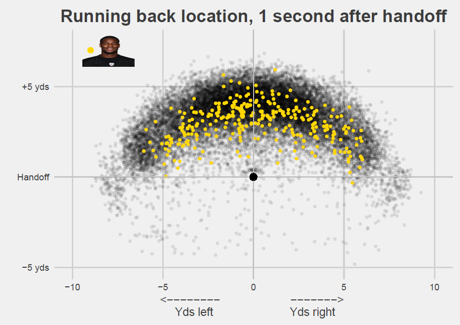
RB locations
Big Data Bowl
Background
Football Ops website with rules and winners: https://operations.nfl.com/the-game/big-data-bowl/
(Static) Github page that hosted the data: https://github.com/nfl-football-ops/Big-Data-Bowl
Forthcoming link: each submission, linked with participants and select resumes