How do you estimate outcomes under a set of rules that don’t (yet) exist?
In this post, I’ll walk through how the NFL league office used resampling to estimate metrics related to an offseason proposal related to overtime.
Background
Back in March, the NFL’s competition committee and owners debated the merits of a rule change, proposed by Kansas City, that would allow both teams the opportunity to possess the ball at least one time in overtime. This would create a scenario unlike any other in football. If the game starts with an opening drive touchdown, the receiving team would:
- Need a touchdown to extend the game
- Never punt
- Never attempt a field goal
- Not care much about the clock
Points (ii) and (iii) are key. It is not uncommon for teams to need a touchdown when trailing late, but in those situations, a number of other factors also play a role in decision making, including timeouts, team quality, and game clock.
In overtime, meanwhile, a team needing a touchdown would never punt or kick a field goal. So how often would they score a touchdown?
Resampling plays
We’ll need more granular data than drive outcomes to estimate touchdown likelihood. So, let’s use plays.
One possibility would be to estimate a conditional distribution of play outcomes given down, distance, and field position. That is, given play-level characteristics, estimate the likelihood of gaining certain yardage on the next play. Using that, one could build a drive simulator.
But football’s not that easy. Once you modeled yardage gained, you’d realize you should have started with modeling turnover likelihood. Once you model turnover likelihood, you’d realize you should have started with penalty likelihood. And once you modeled penalty likelihood, you’d realize you should have built a model to estimate where the drive would start in the first place. Basically, a statistics version of “If you give a mouse a cookie”. You could also model a joint distribution here, but, at this point, that’s an area for future work.
In absence of building several such models, a second, simpler approach would use the observed set of plays and some resampling. That is, at each down, distance, and yard line, we’ll sample from the empirical distribution of similar plays to simulate a play that could happen.
Here’s a version of what this looks. Given that our internal data is a slightly more enhanced than what’s out there publicly, for this post I modified our code to accomodate the public play-by-play data from nflscrapr. Each of these plays are stored in a data frame scrapr.plays, grabbed using code here.
Pre-processing
First, to ensure team motivations roughly fall in line with those participating in an overtime game, I’ll strip the entire set of NFL plays into scrimmage plays run in one possession games, outside of the last two minutes of each half. I also drop two-point conversions, create indicator for whether a fumble or interception occured (is.turnover), whether an offensive (is.td.offense) touchdown occured, and add a variable for line-of-scrimmage (yards from own goal, or yfog).
library(tidyverse)
scrapr.plays <- read_csv("scrapr_plays.csv")

df.scrimmage <- scrapr.plays %>%
  filter(play_type == "pass"|play_type == "run", half_seconds_remaining >= 120) %>%
  mutate(p.diff = total_home_score - total_away_score,
         is.two.point = grepl("TWO-POINT CONVERSION", desc),
         is.fumble = !is.na(fumble_recovery_1_team),
         is.turnover = grepl("INTERCEPTED", desc)|(is.fumble & fumble_recovery_1_team!=posteam),
         is.td.offense = rush_touchdown|pass_touchdown,
         yfog = 100 - yardline_100) %>%
  filter(abs(p.diff) <= 8, !is.two.point,
         !is.na(yards_gained))
Sampling plays
Next, I write a function, sample.rp.drive.needs.TD, to sample df.scrimmage based on down, distance, and line of scrimmage. The code for that is here. Given that 1st-10 plays from midfield are similar to 1st-10 plays from, say, the 47-yard line, the sampling process gives a bit of wiggle room around yard line to increase the number of plays available at each down and distance. In this example, I use +/- 3 yards, +/- 2 yards, +/- 1 yard, and 0 yards for (1-70), (71-90), (91-97), and (98-99) yards-from-own-goal intervals, respectively. I don’t want to add three yards when a team has 3rd-goal from the one, but I’m okay sampling a 3rd-5 play from the 40 yard-line when a team is actually at the 42. To allow for larger samples of plays, 4th-down plays are treated as 3rd-downs.
As an example, here’s the type of outcome you’d get from the function above. On one 1st-10, Mitchell Trubisky hits Taylor Gabriel for a 54-yard catch! On the next, Joe Flacco is picked off by Steve Gregory.
sample.play <- sample.rp.drive.needs.TD(down = 1, yards.to.go = 10, yards.from.own.goal = 25)
sample.play$play
## [1] (7:50) (Shotgun) M.Trubisky pass deep left to T.Gabriel to MIA 21 for 54 yards (T.McTyer).
## Levels: (7:50) (Shotgun) M.Trubisky pass deep left to T.Gabriel to MIA 21 for 54 yards (T.McTyer).sample.play <- sample.rp.drive.needs.TD(down = 1, yards.to.go = 10, yards.from.own.goal = 25)
sample.play$play## [1] (7:42) J.Flacco pass deep middle intended for D.Pitta INTERCEPTED by S.Gregory at BAL 42. S.Gregory to BAL 6 for 36 yards (R.Rice).
## Levels: (7:42) J.Flacco pass deep middle intended for D.Pitta INTERCEPTED by S.Gregory at BAL 42. S.Gregory to BAL 6 for 36 yards (R.Rice).Sampling entire drives
We’ll want to iteratively build out drives, so that after each play, the offensive team continues to try and move down the field. After Gabriel’s catch above, for example, the offense would have 1st-10 from the opponent 21-yard line. Note that for simplicity in this post, I’ll assume each drive started at a team’s 25-yard line – in overtime, roughly 70% of drives start here.
The key part of the loop below is the while() command: we continue to sample plays until (i) a turnover (ii) an offensive touchdown or (iii) a team goes for it on 4th-down and fails, any of which would formally signal the end of the drive (end.of.drive).
set.seed(0)
all.drives.store <- NULL
n.sim <- 10000
yfog.start <- 25
for (i in 1:n.sim){
  drive.store <- NULL
  new.down <- 1
  new.distance <- 10
  new.yfog <- yfog.start
  end.of.drive <- FALSE
  play.num <- 1
  while (!end.of.drive){
    run.play <- sample.rp.drive.needs.TD(down = new.down,
                                         yards.to.go = new.distance,
                                         yards.from.own.goal = new.yfog)
    run.play$play.num <- play.num
    drive.store <- bind_rows(drive.store, run.play)
    new.down <- run.play$new.down
    new.distance <- run.play$new.distance
    new.yfog <- run.play$new.yfog
    end.of.drive <- run.play$end.drive
    play.num <- play.num + 1
    drive.store
  }
  i <- i + 1
  drive.store$sim.id <- i
  drive.store

  if (i %% 100 == 0){print(i)}
  all.drives.store <- bind_rows(all.drives.store, drive.store)
}
What a simulated drive looks like
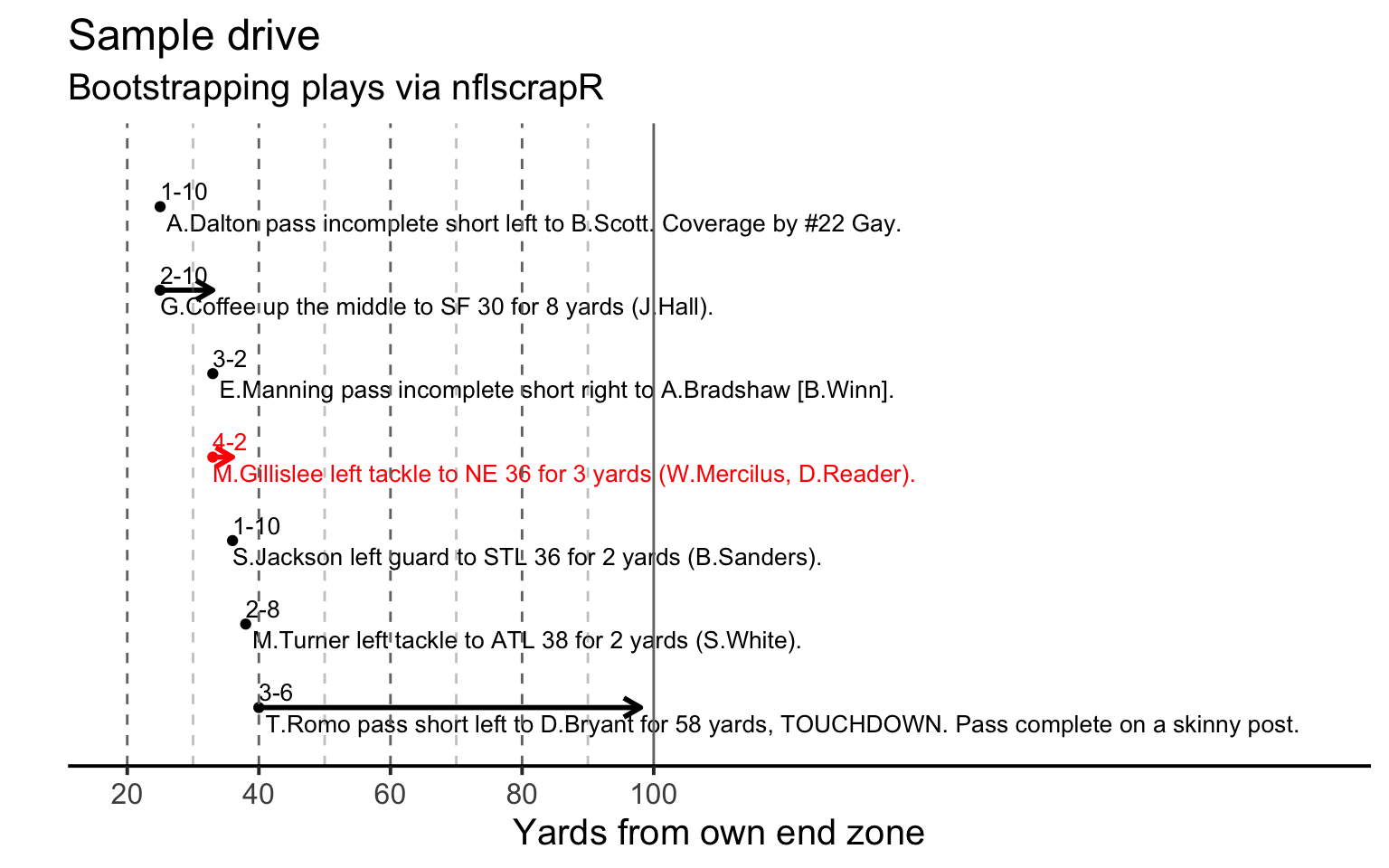
Here’s one sampled drive. It starts with an Andy Dalton pass on 1st-10, and ends a few plays later with a long pass to Dez Bryant. Keep in mind that this should look weird – we’re sampling plays across the last decade of play, and will jump back and forth between offenses.

More importantly, this particular drive shows the importance of replicating what could happen in overtime. Above, the offense went for it on 4th-2 in its own territory, a Mike Gillislee run that is shown in red. In a typical game, most teams in this situation would have punted the ball away. By being forced to be aggressive, what was otherwise a likely punt became a touchdown.
Aggregating across drives
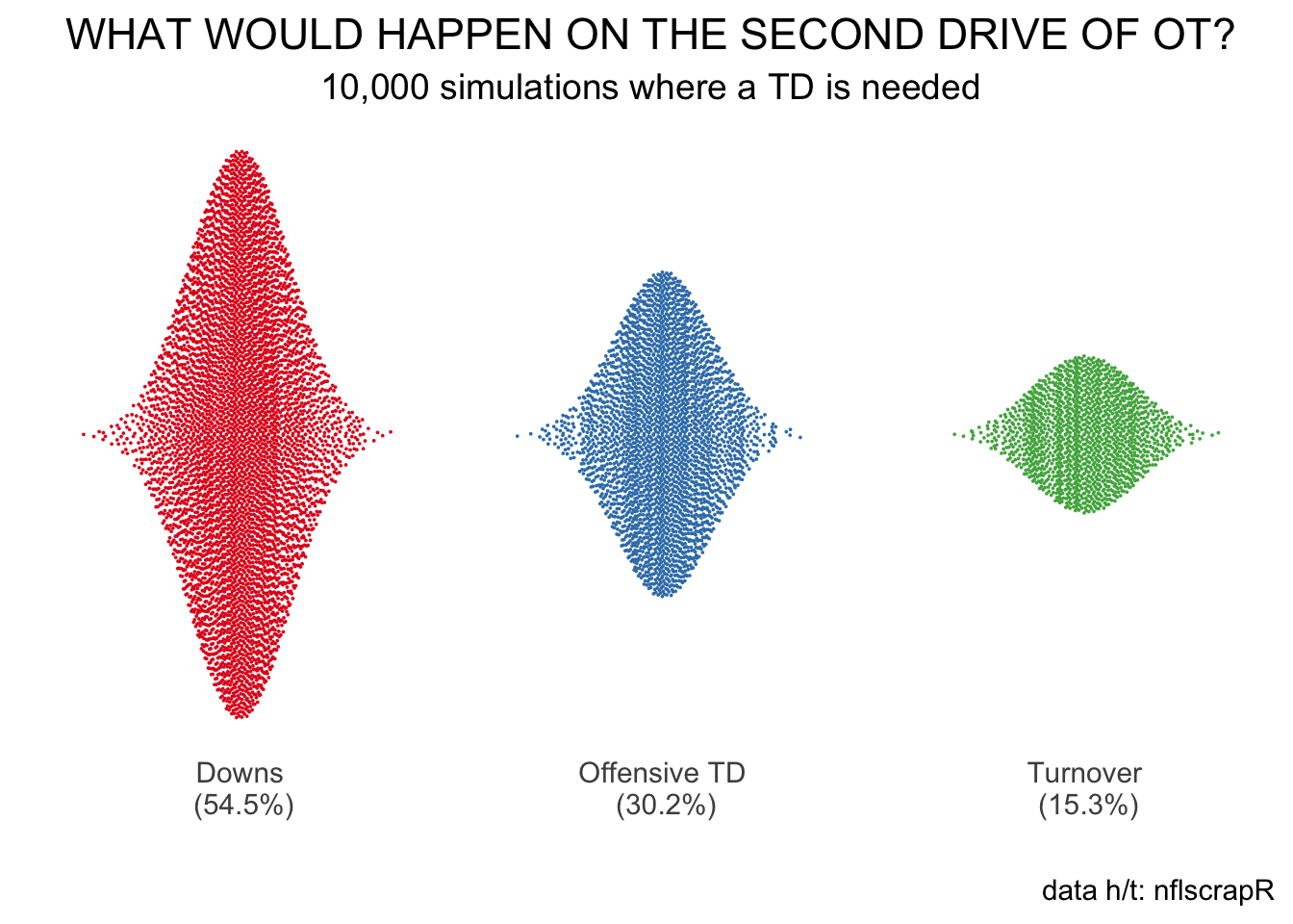
So, how often would an offense score a touchdown in overtime? Here’s a plot of drive outcomes. Each of the 10,000 simulations is a dot, and about 3 of every 10 dots signify an offensive touchdown. In other words, when needing a touchdown and a touchdown only, an offense will score on about 30% of its drives.

How’s this compare to non-overtime drives? Well, teams score a touchdown on the first drive of overtime about 20% of the time, which is roughly what matches the first drive of the game. In other words, the need to score a touchdown increases a team’s chance of scoring that touchdown by about a factor of 1.5.
But wait, there’s more.
The above simulation dodges a few things that complicate football drives, most notably penalties. In our work at the league office, we got a number closer to 40% than 30%. That is, when you add in penalties, which tend to help the offense more than they help the defense, you’ll likely get a rate higher than the 30% I got above. Additionally, changes to the game (recently, more passing) and potential changes in third-down behavior (perhaps teams would run more if they know they are going to go for it?) are two weaknesses that jump out in the above approach.
For now, however, hopefully this gives you a sense of how resampling helped project rules in NFL games that don’t exist. In our case, we sampled from the empirical distribution of actual plays to simulate an offense moving down the field in overtime. Given the forced aggressiveness, we identified a touchdown scoring rate that we could use to better assess what could happen under a rules proposal that would change how NFL overtimes work.